Experts’ voices: 3 years – 3 guys – 3d

March 30th, 2024 | by GEONATIVES

Posted On March 30, 2024

_{(9 min read)}

Hannsjörg started his career as an electrical engineer and, originally, had a focus on acoustics. But, as he put it, he soon “drifted” into visualization. His career reflects the development we see in various technologies, even these days: What begins in a niche with specialized hardware solutions and dedicated chipsets, evolves to become a technology that can run on generalized hardware with specialization and optimization being handled in software. The same domain shift is currently taking place in the automotive industry where the vehicle as an agglomeration of dedicated electronic control units (ECUs) becomes a software-defined vehicle with generalized high-performance computing (HPC) devices.

The 80s

But back to Hannsjörg and the beginning: In the early 1980s, Daimler (what today is Mercedes Benz cars), decided to build a driving simulator in Berlin with a 6-channel visual system developed by Evans & Sutherland. For the ones of our readers, who have not (yet) been around at that time, imagine this endeavor taking place in a pre-Nvidia, pre-Google, pre-GUI, pre-whatsoever setting. Just think of a text editor, 3d coordinates and 256 colors being the only options to define vertices on flat polygons. All the rendering algorithm did was calculating planes with the help of the polygons and adding color and brightness to them for each screen pixel. Impossible, you say? Reality back then!

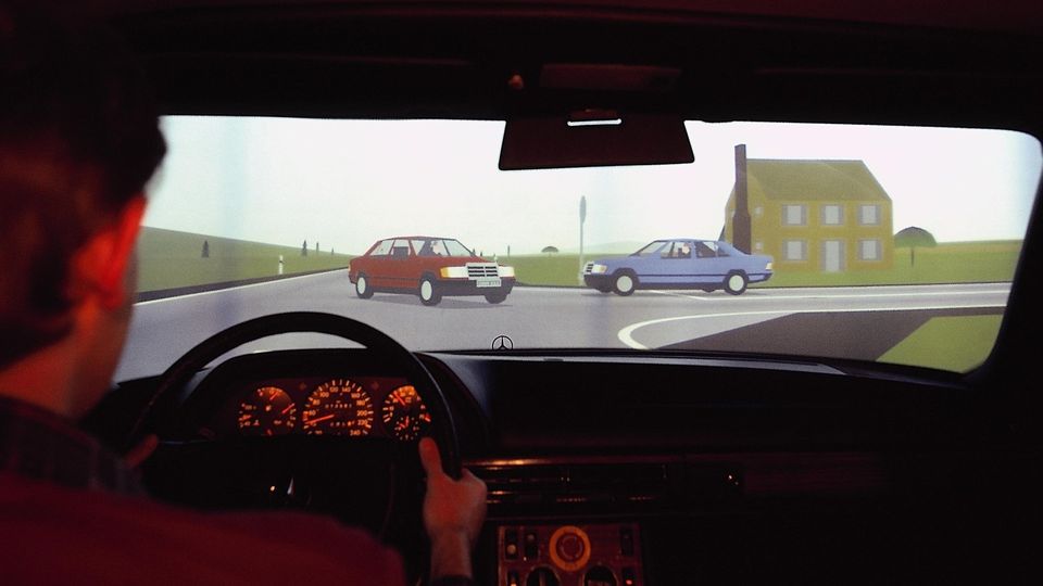
When polygon count matters (images by Mercedes Benz)

Z-Buffering as a solution to the hidden surface problem had already been invented by Henry Fuchs and Ed Catmull, yet, but in the early 1980s it was technologically as well as economically not suitable for higher resolution images. Therefore, artificial constructs like separation planes, for example, had to be included into the 3d data to allow the real-time rendering of a small 4 digits number of polygons per frame. And it had to be precisely defined, what portion of the polygon load could be spent for the road description, including traffic signs and road markings, for other vehicles and for the surrounding landscape.

Hannsjörg worked on custom graphics computers with a hardware-defined rendering pipeline that could generate images of shaded polygons every 25 ms but with a pipeline-depth of 2.5 frames (i.e., it took data 60-something milliseconds to get from input to output). Why would anyone hire an electric engineer for that job? Because, as we already said, it was a hardware-dominated thing. The software was mostly limited to the microprocessor level; the rendering algorithm was baked into hardware. Thus, when something went wrong, the bugs were primarily in the hardware itself.

So, Hannsjörg started his job equipped with a soldering iron, spare boards and sufficient funds to buy COTS microchips and electric parts at a shop in Berlin. That’s the drastically simplified version; but you get it: the software was still too simple to cause much of a spontaneous trouble. Failures during operation were almost exclusively hardware failures. As Hannsjorg put it, this situation made him a bit nervous at the beginning but after having become proficient in diagnostics and locating the exact board or part that had to be replaced based on recognizing faulty image patterns, he practiced it as some kind of art. The saying has it that he has even impressed the late Prince Philip with his skills upon his visit to the driving simulator in Berlin.

Geodata back then

Apparently, the data rendered were roads and vehicles. But what did the geodata look like and how was it created? Today, we talk about laser-scanning real environments, converting point clouds into 3d meshes on centimeter accuracy level, and associating material properties with each little detail. Back then, road and environment were, literally, defined as co-ordinates in a text editor. Light-effects were emulated by associating different vertices of polygons with different colors and having the system interpolate between these colors (so-called gouraud shading). Textures had not yet been invented.

How did you make sure that your geodata was defined correctly and that you had no typos in your coordinates? The first visual system Hannsjörg had been working on, was a singleton, i.e., there was just one system integrated into the simulator and it had to run for actual engineering work to be conducted. A second system for preparation, even with just one channel, would have been “ridiculously” expensive. Therefore, the (not-to-be-envied) colleague who was defining the 3d content had to work asynchronously of the other team members and had to spend the times when they were, for example, having lunch break loading his data into the system, analyzing what he saw, taking notes on a paper clipboard and correcting the data in his text files.

No wonder, it took months to get small stretches of what categorizes as geodata – but sure isn’t comparable with what we associate with them today – into the system. It also took up to nine months to get a car model defined in the system in the same way.

Invention usually comes when resources are scarce. Therefore, since the system definitely didn’t allow for geo-specific databases to be created for specific tests within reasonable time, a library of generic tiles (each 4×4 km² with standardized connections) was created. As dictated by real-road construction rules, the roads were based on straight as well as curved sections and linked by clothoids. All of this was accompanied with some surrounding landscape. From the library, instances of tiles could be configured and combined per test, so that long stretches of motorway or cross-country roads could be created and even linked to each other.

This concept was a key strength of the simulator and was preserved even into the modern-day era. Why? Because not all tests need to be carried out in geo-specific environments. Actually, the geo-specific simulation is just a fraction of what can be done on a simulation “monster” like a dynamic driving simulator the size of the one Hannsjörg worked on (here’s a link to a later version of it). If you are concentrating on tasks like usability, vehicle dynamics, handling, driver fatigue and the same you will have specific requirements for the sequence of road elements that you want to experience (e.g., multiple left-turns or motorway entrances and exits). This is nothing you will find in exactly the same order in any given real location. And bridging the distance between simulated real locations in a simulator might be a distraction that will interfere with your experiment, ultimately. The simplified graphics (compared to nowadays possibilities) are already enough to make the test person emerge in the driving task and reproduce realistic results and behavior.

However, sometimes real-world tracks were requested. For that, planning documents on paper got manually converted into co-ordinate representations for the simulator.

There’s another interesting point in the tile concept that gives a clue about the real background of driving simulation: aerospace or, more precisely, flight simulation. There’s no way around crediting military flight simulation with inventing some of the key elements of what we still use today.

The tile concept is one of these elements. And you can easily imagine it being used to cover large stretches of cross-country flight over mostly amorphous terrain that cannot be loaded at once into the memory of the image generator but needs to be paged in and out as necessary. Points of interest (e.g., airports) are represented by tiles of higher detail, whereas the parts between them are more generic.

The advances in visualization hardware are another element. Purchasing and operating image generators in the old days required deep pockets. Only a few commercial companies like Mercedes, where Hannsjörg worked, were able to afford these instruments. But the majority was deployed in military flight applications.

And, finally, together with advanced hardware came advanced tooling. But from the functionality the tooling provided, you could clearly see it had originated in aerospace applications.

The 90s

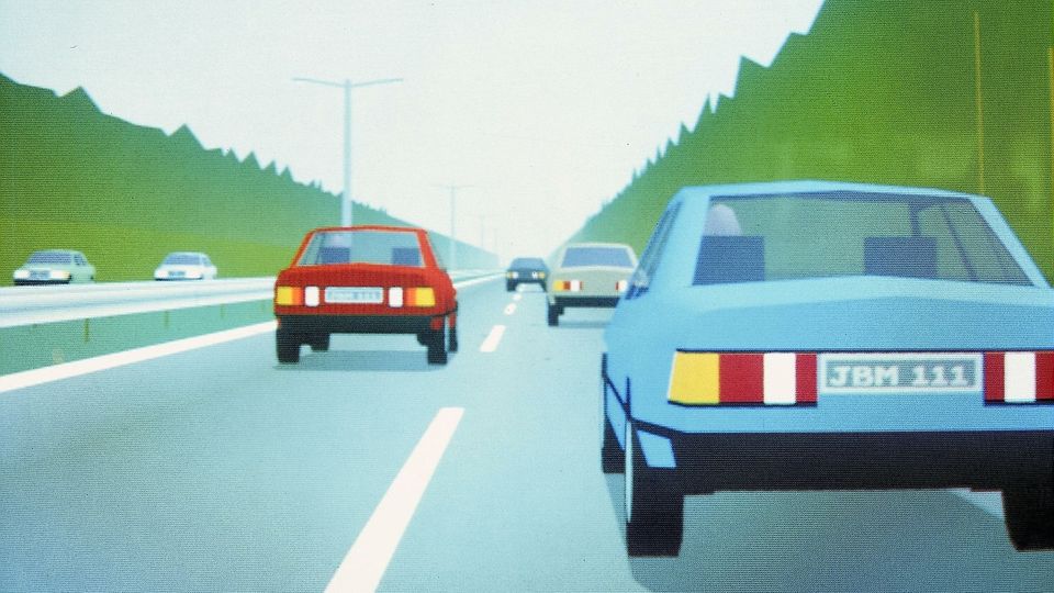
The nineties brought lots of advances. With the next generation of image generators, the rendering pipeline was still carved in hardware, but it came with new features like textures. It could even apply different layers of textures such as color and structure textures that got blended or could be switched, so that it was possible to texture a database for different seasons.

Size of texture memory was still marginal compared to what we have today, but by combining low-resolution color images with higher resolution greyscale images, an unprecedented perception of detail could be achieved. Again, this technology had emerged from military flight applications with aerial imagery starting to make it into the systems.

Another big step came when the first interactive editors for 3d databases became available. Hannsjörg reminded us of the days of “MultiGen” by “Software Systems”, a Silicon Valley company (later operating under the name Presagis and now part of CAE). This was, indeed, a graphical 3d editor that could perform live rendering of simple, textured artefacts. It required another instance of an image generator on which it could run but since hardware costs came down, also this could be afforded as the productivity gain outweighed the investment. That the new software led to some people struggling to operate a computer mouse in additon to a dial box for the first time in their lives, is another story.

See the team in operation in a video on YouTube.

Geodata got somewhat organized in the 90s. Two source data formats prevailed: Digital Terrain Elevation Data (DTED) and Digital Feature Attribute Data (DFAD). Both being of military origin didn’t allow civilian use, but they defined a split in data that we still see today in layered concepts: the long-term static part and the more variable – but not yet dynamic – part. Buildings, vegetation, infrastructure elements all were to be placed on the terrain that was given. Editors like MultiGen were designed to import the DTED and DFAD data and create “nice” databases from them. The long-term static part was created offline based on various aerial surveys and the more variable parts were updated online based on intel.

What MultiGen also brought, was a hardware-vendor-independent database format for visual databases: OpenFlight. It was the first time visual geo databases could be created independently of the actual image generator. This opened the market for other players to provide solutions (either from rendering side or from content side) and helped pave the way to what we have today: a full ecosystem of simulation software and hardware at affordable costs.

At that time, even the idea of a “world database” came up where people dreamt of all parties which were editing databases for different parts of the world combining their data and, thus, covering large parts of the “virtual” globe. A project never took off, and it would be courageous to call this the initial idea for Google Earth, but the similarities are significant.

Going geo-specific

Remarkably enough, Hannsjörg and the driving simulator team he worked for, stuck to the tile concept of generic road elements. They updated and re-engineered their databases along the advance of the technology but never gave up on the basic principles: 4×4 km² tiles with standardized interfaces.

Real tracks made it into the simulator, too. After the simulator team had been relocated from Berlin to Sindelfingen and had built a new, even larger dynamic driving simulator there, the request came up to resemble roads in the neighborhood of the plant that were used for actual test driving as digital twins in the simulator.

Precise surveying of roads made accurate real-world tracks available for driving simulators. The requirements for visual and physical accuracy were high and it took quite a while to get a database done, including lots of hours of debugging for visual inconsistencies and tuning of performance under the load of additional “traffic”. The editing of databases, therefore, was somewhat a step back compared to the productivity level that had already been achieved with tiled databases. And connecting the real-world pieces with the artificial tiles from the catalogue made adaptor tiles necessary to meet the transition points.

But, on the other hand, management likes nice virtual environments. Nevertheless, the focus is still on synthetic roads satisfying the needs of the research question.

Today

In our interview with Hannsjörg, we were most fascinated by stories about the “old days” and on the origins of driving simulation in flight simulation. Where the latter was mostly about flying over terrain, driving simulation was and is fully immersive with lots of interaction with nearby objects.

What we have today is an unprecedented performance and flexibility of hardware and software, communities driving open-source projects and digital twins of hitherto unbelievable precisions. But under the hood, the principles laid in the 80s and 90s still apply.

Geodata has made it into applications far beyond military flight operations and hasn’t stopped in driving simulation even. It goes into apps for everyday use in our mobile phones and provides access to augmented information like, for example, in the “Stolpersteine App” (stumbling stone) or digitalizing our environment and assets such as graveyards or cities to make information available for everybody.

Thank you

A big thanks to Hannsjörg for spending his evening with us on the interview that is the basis for this post. Hannsjörg has retired from Mercedes Benz in 2019 after more than 35 years in the business of visualization for driving simulation.

Or, to put it into terms more familiar to this industry: Hannsjörg spent more than 66,225,600,000 (66 billion) image generator frames (@60Hz) of his life, exploring distorted and undistorted channels, and handling synchronous and asynchronous tasks without getting fully frame-locked and still showing a capability to enjoy a colorful life in stereo after all. How much more can one wish for?

Thanks again!