Geodata for Railroad Simulation
June 9th, 2021 | by Marius Dupuis
(14 min read)
In this post, we want to shed light on geodata for railroad applications with a special focus on simulation for driver training. Engineering simulation is another use case, and the big difference is that engineering will shape reality whereas drivers and operators will consume it. Beyond that, they all rely on the same mechanisms and models. Let’s get started:
Simulation for Advanced Driver Assist Systems and Automated Driving is among the most prominent applications where geodata is processed these days. But if you look at the early adopters of simulation with a need for geo-specific content, there is hardly a way around aerospace and railroad applications.
Simulation has been part of engineering applications and driver training in railroad operation for the past 25+ years (the author was personally involved in his first projects in 1996). Where once novice drivers were educated on-the-job by experienced colleagues, it became mandatory in terms of safety and scarce availability of slots on actual tracks to transfer a good part of driver training to simulators.
Early adopters in this domain were major railroad operators like Deutsche Bahn but also tram and metro operators around the globe. Not only did they require virtual training means for existing routes but also familiarization in advance for routes that were still under construction and had to be operated at full throttle from the very first day of availability. How else but with early incorporation of (projected) geodata could drivers be made familiar with not-yet-existing environments in a virtual installation?
No matter whether training is conducted on virtual representations of existing or projected tracks: using simulators for driver training in the railroad context comes with a couple of other benefits. Drivers can be trained and tested for actual performance in a whole series of rare, dangerous situations that they would otherwise only experience by chance during regular training. And they can fail and gradually improve their operation of the equipment without raising any safety issues.
A Layered Approach
Back to geodata. We need to shed some light on the composition of railroad infrastructure. Much effort has been put by scientist in layered concepts for automotive applications (see [1]-[4] in the references) in recent years. We want to use these results and try to apply them to the railroad case.
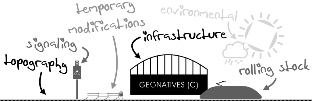
Topography
In a first layer, you find the topography of the railroad tracks. Depending on the age of a route (passenger transport started in 1825!), the corresponding data are either available as paper-only version of the blueprints that were used for constructing the railroad track in first place or they are already digitized and, therefore, available as digital versions of the paper copies or genuine CAD data.
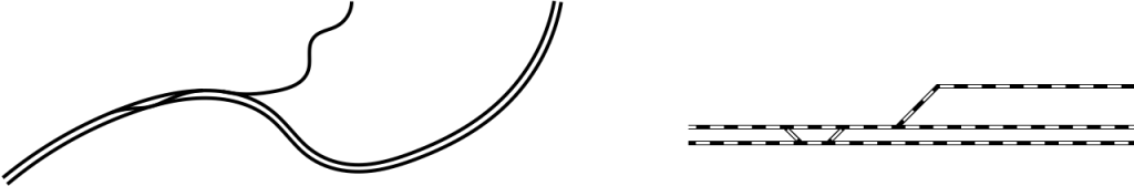
No matter what the format may be, you will see that the topography of railroad tracks comes in highly detailed form with information about segments that are either straight lines, arcs or transition curves (so-called spirals or clothoids). A key property of (most) mainline railroad tracks is that they are laid out with continuous curvature with optimum ride comfort for passengers – in contrast to tracks in mining, agriculture or production plants (your iron ore won’t care about ride comfort aspects).
This is quite different from roads where your vehicle provides one more degree of freedom – the steering. The steering angle determines the curvature of an arc that a road vehicle will follow. A driver will typically not provide steering input as a step function but as a continuous rotation of the steering wheel. Therefore, curvature will be changed continuously and any deficiencies in road layout will automatically be compensated for. This doesn’t mean that roads, especially the ones with higher layout speeds, don’t provide elements of continuous curvature; and if you follow them exactly, you will definitely experience a smooth ride. But the road surface is just the space where a driver may choose an individual path and still experience continuous curvature.
Not so in a train. You will have a hard time locating the steering wheel in a train set. Curvature is imposed onto a train by the track. But this means that continuity of curvature lies only in the construction of the track itself.
When simulating a railroad track, it is therefore important to replicate exactly the curvature information provided in the track plans for two reason: first, the ride comfort in motion-based driving simulators would otherwise be far from acceptable (discontinuities in curvature are translated into hard lateral impact that may damage the equipment or, even worse, cause injuries of the trainee); second, railroad tracks are frequently running in parallel, and getting curvature wrong would create diverging tracks. If your driver training relies on exact replica of the real world for familiarization of students with their operating environment, this second aspect may directly influence the quality of the driver training and the acceptance of simulation as a substitute for real-world driving.
Railroad switches are other elements of particular interest in terms of curvature. In changeovers, they introduce high curvature over a short stretch of track (in opposing directions on both ends – exceptions apply). A distinction is made between high-speed switches which guarantee continuous curvature (by providing clothoid elements) and have a length of up to 180 m, as well as “standard” switches that introduce discontinuity in curvature and have, thus, substantial influence on maximum speed and ride comfort (just remind yourself of the last train ride where you could feel the difference between switches in open-track and the ones in stations).
There are two more properties that need to be replicated from the plan view information of a track – elevation and superelevation. The elevation profile has strong influence on the overall performance of a train set – for acceleration and for braking. Compared to road vehicles, ordinary trains are no champions at climbing steep hills. Mainline tracks with a slope of more than 2.5 percent are considered steep (for secondary tracks, the value is 4.0 percent) and dedicated operational regulations may apply. Maximum slope of railroads based on adhesion is close to 12 percent, and with geared trains, “the sky is the limit”.
Superelevation will compensate for curvature. Trains are typically put on a quite narrow gauge if you compare it with their rather high center of mass. Therefore, curves are the main factor when it comes to laying out the maximum speed of a train set on a given track. In order to achieve higher speeds in (narrow) curves, banking of the track is introduced in correspondence with its curvature (i.e., changing within spiral sections, constant in arc sections). In general, the banking is limited to 6.5 deg for standard gauge. Tilting trains can add up to 8.6 deg on their own.
As with curvature, superelevation needs to be continuous otherwise your track will provide hard edges. It is also important to know around which axis superelevation is introduced since this strongly influences not only the lateral but also vertical acceleration experienced by a train set and, thus, the passengers in it. (Side note: if you look at roller coasters, superelevation of a track is introduced around a so-called heart curve which means that a point close to the human’s heart experiences minimum translational offset; this reduces the risk for dizziness quite a lot and allows for higher speeds and turn rates around the longitudinal axis).
In summary, the first layer of information with curvature, elevation and superelevation is the one that determines which target location you are going to reach from a given start point by applying the data in a chained calculation. If you get any data wrong in the first layer, not only will your track layout be screwed up but potentially also the comfort and experience in a driving simulator.
And, just to add from the author’s experience, the quality of any track data held in digital form really matters. There was one project where digital data of supposedly parallel tracks was provided by an operator; digitization had been carried out using original paper plans and some “fancy” other sources. Once injected into the typical geometric formulas, though, the tracks came out at two almost opposite locations within the country that were roughly 600 km apart. One track even managed to make a 1,200 deg turn at some point. Impressive and fun to watch but not good at all for any engineering task. Therefore, as laid out in our feature about the processing tool chain, quality assurance of any digital data is the key to making them valuable.
Signaling and Routing
In the second data layer you will find all information about signaling and route management. This layer provides the safety of railroad operation and it tends to be rather complex. In a comparison of road and railroad networks, you will easily see that the clarity of routing provided in railroads (no means for lateral deviation from the tracks, routing controlled by switches) is easily compensated for by the complexity of the signal system. In contrast, road networks come with rather simple signaling but complex routing options – including individual negotiation of priority in intersections etc.
Trains “on the move” tend to have considerable momentum and too little friction for hard braking performance. It may take them well above one kilometer to come to a full stop even in emergency braking mode (an ICE3 train set requires roughly 3 km to go from 300 km/h to 0 km/h in emergency braking mode). Therefore, train drivers rely on early indication of any requirements for adjusting their speed.
Here, the topography of the track comes into play again. The train driver needs to be able to identify a signal’s state within a (visible) distance sufficient for applying normal braking action at the track’s design speed. Curvature and track-side environment (buildings, vegetation, tunnels) will usually reduce visibility of a signal below minimum braking distance. For this reason, repeater signals are introduced at appropriate locations before the actual signal becomes visible so that a driver can prepare for the main signal’s state. The number and designated positions of these repeaters are highly depending on speed, visibility and, thus, topography of a specific track – hence a good case for making sure that geodata is correct and up to date when planning the signals on a track. And if you want to go faster than 160 km/h physical signals have to be replaced by cap signaling.
Signaling is a straightforward task on open tracks, but it becomes rather complex if you take the routing into account. The main purpose of signals is to protect conflict areas. And once you introduce switches in your track layout, you create many potential conflicts between different train routes. Consequently, your track and signal data will not only contain information on signal types and positions but also dependencies of signals on each other and on the commanded routing. This gets kind of interesting in large networks.
These inter-dependencies of signals and routing and their impact on operational safety, are one reason why most train operations are managed by control centers (remember that a train does neither have a steering nor is a mainline train driver entitled to modify the states of signals or switches – exceptions for trams and in shunting areas, depots etc. aside). Operators in these centers are the actual “masters” of safe railroad operation. Not only do they monitor and control the routing of the trains (which is derived from timetables and determines the states of signals and switches). They may also directly command individual elements of the signal and routing system and override their states or instruct train drivers to perform actions that appear inconsistent with, for example, a signal’s state. In other words: any safety inherent to a system will ultimately rely on these operators (and the world press is not short on reports of cases where this did not work).
A Complex Digital Twin
In order to perform their job, operators need two things: awareness of the traffic situation and a thoroughly correct digital twin of the static railroad network they are controlling. For the network, however, they don’t need so much a realistic representation of track topography as an exact representation of “operational space” – given by the topology. Curvature, just to name one feature, is irrelevant to the operator. The sequence and length of sections, though, that determine the potential space to which train sets may be assigned and the speed restrictions are key to running smooth operations and maximizing track capacity.
This raises the topic of different views on the same digital twin. For train drivers, the “naturalistic” view is important, for operators, the “schematic” view reduces complexity and workload. One of the tasks when managing the digital twin, therefore, is to establish processes to create both views from one data set and keep them consistent in all aspects.
In summary, a real-time digital twin is required that reflects all details of the situation “out there”. On top of the static track data, dynamic data (i.e., signal and rolling stock states) will be represented. These must be collected by trusted sensors and transmitted by reliable communication means (i.e., the modern versions of the good old levers and cables). Any error in the representation may result in fatal accidents.
This challenge becomes more impressive if you take, again, the long history of railroad operations into account. Depending on the age of routes and the need for including them in moderately or highly frequented networks, you will find several generations of signaling systems close to each other. In Germany, for example, you may still find so-called “form signals” (which originate from the lever and cable ages), various generations of light signals called punctiform train influencing and ETCS/GSM-R (see below) called continuous train control controlled routes. Now imagine the “fun” of defining the data lake of a digital twin representing all of these variants and keeping them available in real-time.
Temporary Modifications
Routes need to be maintained and temporary restrictions may apply for various reasons. These are best contained in a third layer. This layer will usually not alter the underlying structure and data but it may change the attribution (e.g. speed) or add elements like safety barriers, temporary signals, locks on switches etc.
Interaction with layer three requires special attention by train drivers since it may not be part of regular daily operation but creates zones of high risk nevertheless. For this reason, it is quite natural that elements of layer three are welcome “challenges” for training drivers in simulators.
Local Rules Apply
Before we briefly look into additional layers, let us add one more fact: railroad operation is a highly fragmented business with many local rules and widely differing signaling systems (we already have 16 different types in Europe). Therefore, there is nothing like a generic blueprint for operation. The way railroad systems are operated depends on the individual operator and on the level of sharing infrastructure. Try to compare any two self-contained metro systems even within a single country, each run by a dedicated operator; you may soon realize that the only common denominator might be the track gauge – if at all.
Signals come in different shapes. Light point positions and light point colors are assigned “arbitrarily” (there is something like a common understanding that a red – or magenta – light should not be passed, though), signs may or may not indicate speeds, signal IDs, track features (e.g., curvature, slope), and signal repeaters are positioned and denominated according to different rules etc.
Therefore, in a continent as densely populated as Europe and with many countries running quite different railroad operations, it is crucial that rules be unified. Otherwise, journeys going from one country’s capital to another one’s will only be possible by changing trains at the border or, as was one solution in the past, by changing the locomotive (side note: for the particular issue of different gauges, “exotic” solutions like the Talgo III RD (operated until 2010) and Talgo 250 HSR (still in operation) train set with variable gauge axles are used). The introduction of multi-system locomotives that are capable of working under various conditions enabled smooth operation across borders but at the expense of increased complexity. Thus, standardization and alignment of the systems is mandatory. The key initiative in this respect is the so-called European Railway Traffic Management System (ERTMS). Within its framework, railroad operations across borders shall be facilitated and complexity shall be reduced.
With this, your digital twin may gain another layer of complexity since you may have to represent various countries’ local properties plus the European one. But, after all, it is a chance to simplify everything in the long run.
Three More Layers
Now for the additional layers: infrastructure and surroundings, rolling stock, and external influences.
Infrastructure is everything along the tracks that is part of railroad operation but not of signaling. Therefore, halt signals or shunting signs are part of layer two, but catenary, noise barriers, station platforms, human-made structures and the natural environment are part of a fourth layer. They are no less important, though, since they may influence layer two (you have to put signals at locations with minor or no occlusion) or the operation itself (some drivers may use landmarks or features for orientation, see below).
Layer four is the last one of primary interest in terms of geodata. And it is the one where different stakeholders get involved for sure, finally. You have to collect and inject data from railroad operators (who are usually responsible for stations, shunting areas, power distribution etc.), from operators of other transport means (e.g. for making sure that you get a complete routing across various service options with guaranteed connections) and from municipalities, land registers, counties, states etc. Rail lines tend to “cut” through other parties’ areas of interest, and harmonization of data in each party’s digital twins is crucial. Just imagine the need for negotiating the position of a railroad crossing among all interested parties; or planning for monitoring the growth of vegetation along a track so that trees are cut early enough in order not to be felled by an occasional storm and, thus, blocking the tracks. Ideally – and favored by us – there will be only one digital twin, though, which is accessible to all parties and maintained in a well-defined process.
We already talked about layer five without mentioning it explicitly. Here, you will find the rolling stock with time-variant positions of each entity. This is, naturally, the most dynamic layer that must be kept up to date (in terms of seconds!) for safe operation of a railroad network. It directly interacts with layers one and two since occupation of a track segment by a train set is reported by track-side sensors or digital radio-based (or, in legacy systems, by a station’s head who is monitoring traffic and manually controlling signals in his area of influence by pressing fancy buttons – you dearly hope not to run on this kind of network anymore but you are doing it more often than you expect).
Signals and signal states are reported into the rolling stock either by magnets that prevent a train from running a red light (applying auto brake), by telegrams from linear train influencing cabling or so-called balises (see ERTMS) or by GSM-R or GPRS that provide not only signal states but also higher-level information directly to the train driver’s desk.
Finally, in layer six, you will find time-variant external influences on train operation. This may, most prominently, be the weather with its potential deterioration of signal visibility and slippery rails – either by particles like rain, snow and fog or by oncoming sunlight – but also hazards like fallen trees or frozen switches etc. All of them may determine whether and how you can operate your railroad network.
Back to Simulation
Going back to the original topic of this post: simulation.
For simulation, a digital twin is required so that students or engineers experience an exact replica of the actual situation in the real world for their specific use cases. Where for railroad operation centers the emphasis for the digital twin is on safety-relevant features (i.e., signals, switches, power feeds), railroad simulation systems will need to replicate all details of layers one to six. Only with these data will it be possible to create a credible replica of reality that provides sufficient immersion to a student or insights for an engineer.
Just to give one final example: the author was frequently challenged with providing simulations that created exact conditions of on-coming sun light as train drivers would experience them most prominently on east-west bound open tracks. This implied that simulated tracks were geo-located correctly, that the ephemeris model allowed for specifying time and date of the simulation and that environment features were causing correct shadows or stroboscopic effects.
This orchestration makes an excellent example of a data lake that is composed from various sources (track maps, environment scans, traffic and weather statistics, operational data like timetables etc.) and which is exported with varying extent for different use cases (simulation and actual railroad operation) and stakeholders (railroad operator, municipality etc.).
Consistency of data across all target applications and between the targets and real-world data is a must. Therefore, the goal has to be one lake of trusted and up to date data that can be applied seamlessly to all targets.
To be Continued – How to Organize the Data
The big remaining question is how to structure the data lake and what formats to use so that it can fulfill its purpose. For this, we refer to an upcoming expert interview. We will sure let you know when it becomes available on our website.
Conclusion
Data for railroad operation and simulation comes in different layers. Starting with track geometry and supplemented by signaling and surrounding infrastructure data, the operational basis is well defined. Information about rolling stock and external influences complements a six-layer model that has to be fully implemented for the simulation of railroad operation – either from a train driver’s, a traffic controller’s or an engineer’s view (or all at once).
Different use cases require that data be acquired, verified, held and updated in a data lake that allows for the extraction and conditioning for use cases at varying frequencies. Daily operation will need to be provided with information as well as infrastructure planning, upgrading of signal systems etc.
This feature provided the basis for further discussion of various topics in the field of geodata for railroad operation and simulation. Stay tuned for more.
References
[1] F. Schuldt, “Ein Beitrag für methodischen Test von automatisierten Fahrfunktionen”, Ph.D. dissertation, Fakultät für Elektrotechnik, Informationstechnik, Physik, TU Braunschweig, Braunschweig, 2017.
[2] G. Bagschik, T. Menzel, and M. Maurer, “Ontology based scene creation for the development of automated vehicles”, 2018 IEEE Intelligent Vehicle Symposium, 2018, pp.1813-1820.
[3] J. Bock, R. Krajewski, L. Eckstein, J. Klimke, J. Sauerbier, A. Zlocki, “Data basis for scenario-based validation of HAD on highways”, 27th Aachen Colloquium Automobile and Engine Technology, 2018
[4] M. Scholtes, L. Westhofen, L. Turner, K. Lotto, M. Schuldes, H. Weber, N. Wagener, C. Neurohr, M. Bollmann, F. Kortke, J. Hiller, M. Hoss, J. Bock, L. Eckstein, “6-Layer Model for a Structured Description and Categorization of Urban Traffic and Environment”. 2021. IEEE Access. PP. 1-1. 10.1109/ACCESS.2021.3072739.